6.2 Parcel data

Parcels are boundaries of land ownership in the U.S. and a key layer of administrative data and regulation in local jurisdiction. This data is notoriously difficult to acquire and standardize for an entire urban region. Generally, parcel geometries themselves are maintained by a County Assessor office and made available for download online. However, these sources don’t tend to hold much information besides the Assessor Parcel Number (APN). The most useful data to attach to parcels are:

• Zoning, a local Planning Department’s regulations on what land uses are allowed on the parcel, which tend to be stored in separate files which may not be available to download online
• Assessor-Recorder Office data, which include ownership and property tax information, as well as building characteristics which would have been collected by the Assessor-Recorder’s Office for the purpose of conducting assessments.

It is generally difficult to publicly access both of these sources of data for a jurisdiction; in particular, the Assessor-Recorder data tends to be monetized by Assessor-Recorder’s Offices or private companies, even though much of it should technically be public record.

For our purposes, we’ll focus on the City and County of San Francisco as a rare location that makes much of its Assessor-Recorder data publicly available through its Open Data Portal, along with zoning. But even for SF, as will be a key theme of this section, be prepared for a lot more data wrangling than you’ve encountered before, because of the inherent messiness of this scale of administrative data.

library(tidyverse)
library(readxl)
library(tigris)
library(sf)
library(leaflet)
library(mapboxapi)

mb_access_token("YOUR_TOKEN_HERE", install = T)
readRenviron("~/.Renviron")

First, let’s read the shapes of parcels from one dataset on the Open Data Portal, “Parcels - Active and Retired”. The approach we’ve used in the past, with the “API Endpoint” URL, appears to only provide the first 1000 rows, so instead I’ve used the URL available under Export > GEOJSON. I’ve also filtered to “active” parcels, and selected the only fields we might need at this stage: APN, zoning code, and zoning description.

sf_parcels_shape <- 
  st_read("https://data.sfgov.org/api/geospatial/acdm-wktn?method=export&format=GeoJSON") %>% 
  filter(active == "true") %>% 
  select(
    apn = blklot,
    zoning = zoning_code,
    zoning_desc = zoning_district
  )

Next, let’s read Assessor-Recorder secured property tax roll data. There are some versions on the Open Data Portal, but they are not updated with the most recently available property data, which is instead found on the Assessor-Recorder’s own website (it is still very notable that SF’s Assessor-Recorder Office makes this data available for download at all, but the activities of this Office do not appear to be fully coordinated with the overall open data ecosystem yet). The link found at this site is an Excel file, so we can use a technique we used in Section 2.2:

temp <- tempfile()
download.file("https://sfassessor.org/sites/default/files/uploaded/2020.7.10_SF_ASR_Secured_Roll_Data_2019-2020.xlsx",destfile = temp, mode = "wb")

sf_secured <- read_excel(temp, sheet = "Roll Data 2019-2020")
datakey <- read_excel(temp, sheet = "Data Key")
usecode <- read_excel(temp, sheet = "Class Code Only")

unlink(temp)

Keep in mind that excel_sheets(temp) lets you see the sheet names in advance, which you can then refer to in the following calls. But it can be helpful to go ahead and download the Excel file and inspect it in advance to understand what is useful to you. datakey shows what kind of information you can get from the Assessor-Recorder.

datakey %>% select(`DATA NAME`, `FIELD NAME`) %>% as.data.frame()

Let’s now try joining the property tax data to the parcel shape dataframe using APN as a joining field. It turns out that the two datasets do not format this field in the same way; in sf_secured, there is a space in the middle of the APN. We also of course don’t know yet how successful of a join this will be, if there are other kinds of formatting issues at a record level. In the next chunk, we use str_replace() to replace " " with "", and then report a series of sums to check how many APNs sf_parcels starts with, how many APNs are successfully matched from sf_secured, how many records in sf_parcels have zoning codes, and how many of the matched records from sf_secured have zoning codes.

sf_parcels <-
  sf_parcels_shape %>% 
  left_join(
    sf_secured %>% 
      mutate(
        apn = RP1PRCLID %>% 
          str_replace(" ","")
      )
  )

sum(!is.na(sf_parcels$apn))

## [1] 224643

sum(!is.na(sf_parcels$RP1PRCLID))

## [1] 213114

sum(!is.na(sf_parcels$zoning))

## [1] 223887

sum(!is.na(sf_parcels$ZONE))

## [1] 174558

It looks like the APN matching is pretty successful but not 100% complete, so later we’ll filter to just records that were successfully matched from sf_secured so we have Assessor-Recorder information. And sf_secured actually had lots of missingness in its ZONE field, so it’s helpful to use zoning information from the open data platform instead. These kinds of insights are part of data exploration and cannot be predicted in advance, so always it’s helpful to do these kinds of sum checks.

Now, to simplify this analysis for our demonstration, given how large the parcel datastes are, we’ll focus on just three arbitrary census tracts in San Francisco’s Inner Sunset District. This is a transit rich area with convenient access to Golden Gate Park, and which has been the subject of political attention on the issue of upzoning. We’ll use our parcel data to evaluate the degree to which what is currently existing development on these parcels is undershooting what is “possible” to build given zoning, along the measures of floor area, units, and stories.

sunset_sample <-
  tracts("CA", "San Francisco", cb = T, progress_bar = F) %>% 
  filter(
    TRACTCE %in% c(
      "030202",
      "030201",
      "032601"
    )
  ) %>% 
  st_transform(4326)

sunset_parcels <- 
  sf_parcels %>% 
  st_centroid() %>% 
  .[sunset_sample, ] %>% 
  st_set_geometry(NULL) %>% 
  left_join(sf_parcels %>% select(apn)) %>% 
  st_as_sf() %>% 
  filter(!is.na(RP1PRCLID))

sunset_parcels %>% 
  leaflet() %>% 
  addMapboxTiles(
    style_id = "streets-v11",
    username = "mapbox"
  ) %>% 
  addPolygons(
    fillColor = "blue",
    color = "black",
    weight = 0.5,
    label = ~zoning
  )

We are now down to under 3000 parcels. Note that, with the automatic fill opacity settings of leaflet, we can see some parcels are a darker blue. This is a signal of residential or commercial condominiumization, where a property is broken up for multiple owners (with separate APNs). Of course the actual boundaries of ownership make be building wall boundaries in an apartment building, but for administrative parcel data, each condominium APN is typically shown with the boundary of the entire land parcel, which can cause problems for our analysis, where we just want to aggregate certain building information for the whole land parcel. So we’ll need to clean up our data, synthesizing information on these condominiumized parcels. To identify which parcel records are on the condominiumized parcels, we can first use duplicated() to filter to records with duplicated geometry information, but this will not actually retain the first record in each duplicated set, so we then use the geometry field of this interim dataframe to go back and filter the original parcel dataframe:

duplicate_shapes <- 
  sunset_parcels %>% 
  as.data.frame() %>% 
  filter(duplicated(geometry))

condo_parcels <- 
  sunset_parcels %>% 
  filter(geometry %in% duplicate_shapes$geometry)

condo_parcels would be useful for mapping and understanding the condo parcels on their own, but for our larger cleaning effort, we’ll be able to more directly use group_by() and summarize() to synthesize information on these condominiumized parcels.

Before doing, let’s also double check our zoning field to see which zones are included in our set of Sunset parcels, which will affect what information we need to look up in SF’s zoning code for our analysis:

sunset_parcels %>%
  st_set_geometry(NULL) %>% 
  group_by(zoning, zoning_desc) %>% 
  summarize(Freq = n())

Notes:

• “Inner Sunset Neighborhood Commercial [District]” and “Irving Street Neighborhood Commercial District” are two separate zoning designations, but confusingly have the same zoning code. Note that this is the kind of data ambiguity that could lead to incorrect analyses if not caught.
• There are 3 public parcels, which we will not consider in our analysis.
• There appear to be three “RH” zones, and three “RM” zones. However there appears to be one parcel that has both “RM-1” and “RM-2” designation. It’s possible that this means something particular in zoning code, but for our purposes, it presents a data cleanliness challenge that outweighs its possible impact on our results. We can choose to remove this record, or make a judgment call that, if RM-2 is more flexible of a designation, it will govern for our purposes. So we’ll manually convert this parcel to “RM-2” for our analysis.

We won’t end up using the property use information in RP1CLACDE, but I’ll show summary statistics for this field, since current use is often very useful to analyze. Keep in mind that when creating summary statistics for just one field, table() is a fast method.

table(sunset_parcels$RP1CLACDE) %>% 
  as.data.frame() %>% 
  left_join(usecode, by = c("Var1"= "CODE")) %>% 
  select(Freq, DESCRIPTION)

Now, let’s begin cleaning our parcel data, both for the condo issue and the zoning codes:

sunset_parcels_clean <-
  sunset_parcels %>% 
  mutate(
    zoning = case_when(
      zoning == "RM-1|RM-2" ~ "RM-2",
      zoning_desc == "INNER SUNSET NEIGHBORHOOD COMMERCIAL" ~ "INNER SUNSET",
      zoning_desc == "IRVING STREET NEIGHBORHOOD COMMERCIAL DISTRICT" ~ "IRVING ST",
      TRUE ~ zoning
    )
  ) %>% 
  filter(zoning != "P") %>% 
  as.data.frame() %>% 
  mutate(geometry = geometry %>% st_as_text()) %>% 
  group_by(geometry) %>% 
  summarize(
    apn = first(apn),
    zoning = first(zoning),
    units = sum(UNITS, na.rm = T),
    stories = max(STOREYNO, na.rm = T),
    floorarea = sum(SQFT, na.rm = T)
  ) %>% 
  ungroup() %>%
  select(-geometry) %>% 
  left_join(sunset_parcels %>% select(apn)) %>% 
  st_as_sf()

Notes:

• To use the geometry field as the argument in group_by() we need to convert it to character information. st_as_text() happens to be useful for this purpose, converting the data into “well-known text” which is a common, efficient text format for geometry information. I’d recommend this if creating CSVs. The data can then be reconverted to sf geometries using st_as_sf(wkt = “field_name”). In our case, we can instead left_join() back our original shapes at the end.
• In summarize(), we are using first() to get just the first apn and zoning records for each group of condos. We would expect zoning to all be the same for the group, but APNs will be different. For our purposes, we don’t have a particular reason to retain the APN field besides supporting the final left_join(), so it’s fine to hold on to just the first APN in the group, whatever it is.
• For stories, we’re grabbing the max() story number from the group, as it appears based on inspection that the record shouldn’t be interpreted as additive.

Now our dataframe sunset_parcels_clean has just 8 unique zones for us to consider and just one row of information per land parcel. We also have summarized information about the total floor area, total number of dwelling units, and total number of stories on each parcel, available through the Assessor-Recorder dataset. The next step of the analysis involves finding out what the maximum floor area, maximum dwelling units, and maximum stories is for each parcel, given its size and zoning. We’ll need to search through SF’s Zoning Code for tables, as you’ll generally find in zoning ordinances, detailing this fixed numbers or formulas for each zoning designation. Expect this to often be a frustrating experience because zoning ordinances are notoriously dense and convoluted. In our case, we would find the following insights.

Max floor area:

• For Inner Sunset NCD, floor area is limited by a floor area ratio (FAR) or 1.8 to 1, meaning that if we know the lot size (which we’ll be able to calculate using st_area(), we can multiply by 1.8 to get maximum building floor area.
• For Irving Street NCD, FAR is 2.5 to 1.
• For the three RH districts, FAR is 1.8 to 1.
• For the three RM districts, RM-1 and RM-2 are 1.8, but RM-3 is 3.6.

Max units:

• For Inner Sunset or Irving St NCDs, the max dwelling units is 1 unit per 800 square foot lot area, or whatever is permitted in the nearest residential district. For simplicity, we’ll assume the first formula governs.
• For RH districts, the number in RH-1, RH-2, or RH-3 is the max number of units.
• For RM districts, 3 units are allowed, or the following if greater: for RM-1, 1 unit per 800 sqft; RM-2, 1 unit per 600 sqft; RM-3 1 unit per 400 sqft.

Max stories:

• In all cases, heights are governed first and foremost by information in separate Height and Bulk District Maps, which we’ll need to read in from the Open Data platform. The possible options we’ll find are 40ft for the vast majority, and two small commercial areas that allow 65ft or 105ft.
• For the RH districts, residential units are further restricted to just 35 ft.
  
• Many other factors can be involved in reducing height and bulk, like setbacks and daylight planes, but we’ll use these simplified rules for our demonstration. To convert from max height to max stories is partially a question of design, but for simplicity we’ll divide by 11ft to get max stories. This will have the advantage of properly limiting the RH districts to 3 stories in a 40ft height limit district.

Here we load in the height districts, filter to just our region, and find the two special commercial areas. The dataset actually just includes districts that are NOT 40ft height limits, since that’s the dominant height everywhere else.

sf_heights <- st_read("https://data.sfgov.org/resource/h9wh-cg3m.geojson")

sunset_heights <-
  sf_heights[sunset_parcels_clean, ]

factpal <- colorFactor(c("red","blue"), sunset_heights$height)

leaflet() %>% 
  addMapboxTiles(
    style_id = "streets-v11",
    username = "mapbox"
  ) %>% 
  addPolygons(
    data = sunset_heights,
    stroke = F,
    fillOpacity = 0.5,
    fillColor = ~factpal(height),
    label = ~height
  ) %>% 
  addPolygons(
    data = sunset_parcels_clean,
    fill = F,
    color = "black",
    weight = 0.5
  )

Now, let’s produce the extra fields max_floorarea, max_units, and max_stories to append to our existing dataframe. At the same time, we’ll create unused_floorarea, unused_units, and unused_stories, which will be just the positive results when subtracting the max from the current usage.

projection <- "+proj=utm +zone=10 +ellps=GRS80 +datum=NAD83 +units=ft +no_defs"

sunset_parcels_zoning <-
  sunset_parcels_clean %>% 
  st_centroid() %>% 
  st_join(sunset_heights %>% select(gen_hght)) %>% 
  st_set_geometry(NULL) %>% 
  left_join(sunset_parcels_clean %>% select(apn)) %>% 
  st_as_sf() %>% 
  st_transform(projection) %>% 
  mutate(
    lotarea = st_area(.) %>% as.numeric(),
    max_floorarea = case_when(
      zoning == "IRVING ST" ~ lotarea*2.5,
      zoning %in% c("INNER SUNSET","RH-1","RH-2","RH-3","RM-1","RM-2") ~ lotarea*1.8,
      zoning == "RM-3" ~ lotarea*3.6
    ),
    unused_floorarea = ifelse(
      (max_floorarea - floorarea) > 0,
      (max_floorarea - floorarea),
      0
    ),
    max_units = case_when(
      zoning %in% c("INNER SUNSET", "IRVING ST") ~ floor(lotarea/800),
      zoning == "RH-1" ~ 1,
      zoning == "RH-2" ~ 2,
      zoning == "RH-3" ~ 3,
      zoning == "RM-1" ~ pmax(3, floor(lotarea/800)),
      zoning == "RM-2" ~ pmax(3, floor(lotarea/600)),
      zoning == "RM-3" ~ pmax(3, floor(lotarea/400))
    ),
    unused_units = ifelse(
      (max_units - units) > 0,
      (max_units - units),
      0
    ),
    max_height = ifelse(
      is.na(gen_hght),
      40,
      gen_hght %>% as.numeric()
    ),
    max_stories = floor(max_height/11),
    unused_stories = ifelse(
      (max_stories - stories) > 0,
      (max_stories - stories),
      0
    )
  ) %>% 
  st_transform(4326)

Notes:

• We need to use projection because we want our st_area() calculation to be in sqft.
• When we calculate st_area(.), we also pipe to as.numeric() because the area is in a special class called units which won’t immediately work in math formulas later on.
• pmax() takes the highest of multiple values; pmin() would do the lowest of multiple values.

Some summary statistics:

sum(sunset_parcels_zoning$unused_floorarea, na.rm = T)

## [1] 7435047

sum(sunset_parcels_zoning$unused_units, na.rm = T)

## [1] 2063

That’s about 7.4 million square feet of floor area that could be built in this area under current zoning, meaning the land is underutilized to this degree. If all of that underutilized space were to be used for housing, there could be about 2,000 more dwelling units, without changing zoning. Let’s visualize these two results:

floorarea_pal <- colorBin(
  palette = "Greens",
  bins = c(0,1000,5000,10000,max(sunset_parcels_zoning$unused_floorarea, na.rm = T))
)

leaflet() %>% 
  addMapboxTiles(
    style_id = "light-v9",
    username = "mapbox"
  ) %>% 
  addPolygons(
    data = sunset_parcels_zoning,
    fillColor = ~floorarea_pal(unused_floorarea),
    fillOpacity = 0.75,
    color = "white",
    weight = 0.5,
    label = ~round(unused_floorarea)
  ) %>% 
  addLegend(
    data = sunset_parcels_zoning,
    pal = floorarea_pal,
    values = ~unused_floorarea,
    title = "Unused Floor Area"
  )

Note the use of colorBin() to set our own manual breaks for the legend, given the large skew of some outliers with very high unused floor areas.

units_pal <- colorBin(
  palette = "Purples",
  bins = c(0,1,5,10,max(sunset_parcels_zoning$unused_units, na.rm = T))
)

leaflet() %>% 
  addMapboxTiles(
    style_id = "light-v9",
    username = "mapbox"
  ) %>% 
  addPolygons(
    data = sunset_parcels_zoning,
    fillColor = ~units_pal(unused_units),
    fillOpacity = 0.75,
    color = "white",
    weight = 0.5,
    label = ~round(unused_units)
  ) %>% 
  addLegend(
    data = sunset_parcels_zoning,
    pal = units_pal,
    values = ~unused_units,
    title = "Additional Units<br>Allowed"
  )

For unused stories, just for fun, let’s try something fancier. First, we’ll make a ggplot result instead of a leaflet result:

stories_plot <- 
  sunset_parcels_zoning %>% 
  filter(unused_stories > 0) %>% 
  ggplot() + 
  geom_sf(
    aes(
      fill = unused_stories
    ),
    lwd = 0
  ) + 
  theme(
    axis.text.x = element_blank(), 
    axis.text.y = element_blank(),
    axis.ticks = element_blank(),
    rect = element_blank()
  ) +
  labs(
    fill = "Unused Stories"
  ) +
  scale_fill_gradient(
    low = "white",
    high = "red"
  )

stories_plot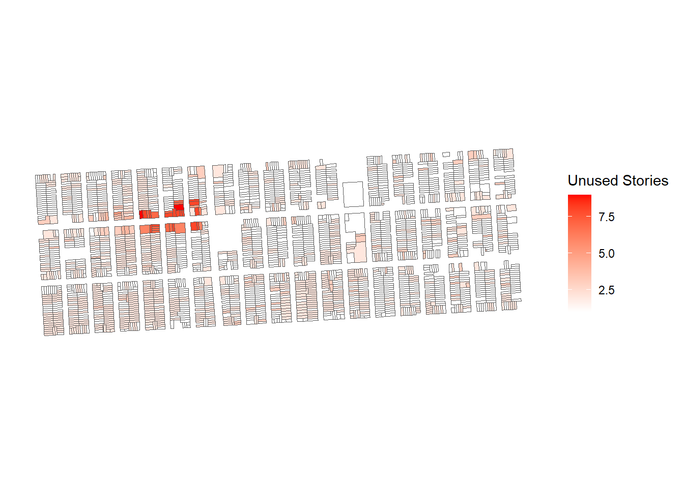

There’s a package called rayshader that can turn ggplot plots into 3D plots. If you run on stories_plot you get the following:

library(rayshader)

plot_gg(
  stories_plot,
  width = 10,
  height = 4,
  scale = 100
)

render_snapshot(
  "snapshot.png",
  clear = TRUE
)

As we would expect, the greatest opportunity for height increases appears to be in the region that had the special height districts. Keep in mind, overall, that this analysis demonstrated opportunity for increased land use between the existing zoning and the existing property use, but this analysis could also be used to estimate development potential for entirely new zoning, which has been a critical consideration at the local and state level.