7.3 Air pollution data
Air pollution data is a key source of information for monitoring and managing one of the primary categories pollutants (air-based) that are caused by our consumption of resources in urban environments. In the Bay Area, besides the impacts of natural hazards like wildfires on air pollution, the main sources of focus would be commercial and industrial point sources, as well as moving sources like vehicle exhaust. If we can identify particular urban areas that are regularly exposed to higher levels of air pollution, such as residences and schools near highways or factories, then we can direct attention to the long-term health impacts of this exposure and target sustainability-oriented (and often equity-oriented) action.
Unfortunately, air pollution analysis has often been coarse, given the lack of air monitoring stations or other kinds of data collection. But a recent company, PurpleAir, is a notable example of a private-sector entity that has made cost-effective indoor and outdoor PM2.5 sensors available to the broad consumer market. In the Bay Area, there are now thousands of PurpleAir sensors, which is giving academics and the public alike unprecedentedly detailed data on air pollution in an easily accessible format. We’ll make use of PurpleAir’s API via a package built by a researcher at Emory University, Jianzhao Bi, bjzresc (which greatly simplifies calls we need to make to the API). We’ll also be using rasters for the first time (to be further explained in the next chapter), so also load stars and raster at this time (which can be installed using the standard install.packages(c("stars","raster"))). Finally, we’ll be performing spatial interpolation with the gstat package, so also install that with install.packages(“gstat”).
library(devtools)
install_github("jianzhaobi/bjzresc")

library(tigris)
library(tidyverse)
library(sf)
library(leaflet)
library(mapboxapi)
library(jsonlite)
library(bjzresc)
library(stars)
library(raster)
library(gstat)
Loading all PurpleAir sensors, including lat/long and some sensor information, is as simple as the following:
Our dataframe shows over 30,000 records total, though many rows are duplicates for one device, given the existence of multiple channels. Next let’s filter to just the Bay Area, based on lat/long. Since the lat/long information from PurpleAir is in the WGS 84 coordinate system, we’ll transform everything to that CRS for convenience in this demonstration.
bay_county_names <-
  c(
    "Alameda",
    "Contra Costa",
    "Marin",
    "Napa",
    "San Francisco",
    "San Mateo",
    "Santa Clara",
    "Solano",
    "Sonoma"
  )

bay_counties <-
  counties("CA", cb = T, progress_bar = F) %>%
  filter(NAME %in% bay_county_names) %>%
  st_transform(4326)

bay_list_air <-
  list_air %>%
  filter(!is.na(Lat)) %>%
  mutate(PM2_5Value = as.numeric(PM2_5Value)) %>%
  filter(!is.na(PM2_5Value)) %>%
  st_as_sf(
    coords = c("Lon","Lat"),
    crs = 4326
  ) %>%
  .[bay_counties, ]
It looks like a significant portion of PurpleAir sensors (over 10,000 records) are in the Bay Area. Now, the PurpleAir dataframe comes with a field PM2_5Value, which, according to the online documentation, is the “current” PM2.5 value based on whenever you read the data. But within a JSON field called Stats, a list item named v6 has a “weekly average”, which will be more useful for our purpose of generally assessing air quality over time. At the end of this section, we’ll demonstrate how to pull even longer historical records than just the past week.
We’ve encountered JSONs before with the SafeGraph data, so in the chunk below, we use the same technique with fromJSON() to extract information from that field. Here, I show map() used within a mutate command; note that the final result has to be an unlisted vector form for mutate() to accept it. We’ll also filter to just “outside” sensors, and also apply a conversion recommended by PurpleAir, produced by the EPA (to better match the composition of pollution expected in a place like the Bay Area, relative to Salt Lake City, where PurpleAir is based).
bay_list_air_clean <-
  bay_list_air %>%
  filter(DEVICE_LOCATIONTYPE == "outside") %>%
  mutate(
    PM25_week =
      Stats %>%
      map(function(row){

        row %>%
          fromJSON() %>%
          unlist() %>%
          as.data.frame() %>%
          .["v6",] %>%
          as.numeric()

      }) %>%
      unlist(),
    PM25_week_EPA =
      0.534*PM25_week - 0.0844*as.numeric(humidity) + 5.604
  ) %>%
  filter(!is.na(PM25_week_EPA))
Now, we are down to just a few thousand sensors. Let’s go ahead and try plotting these as “circle markers” in leaflet, using the “RdYlGn” color palette over a 1:100 domain, which should roughly match the color scheme for the official EPA Air Quality Index:
aqi_pal <- colorNumeric(
  palette = "RdYlGn",
  reverse = T,
  domain = 1:100
)

bay_list_air_clean %>%
  leaflet() %>%
  addMapboxTiles(
    style_id = "streets-v11",
    username = "mapbox"
  ) %>%
  addCircleMarkers(
    color = ~aqi_pal(PM25_week_EPA),
    label = ~PM25_week_EPA
  )
It turns out that at the time of this demonstration (11/1/20), the weekly average for pretty much all of the Bay Area was in well within a “good” AQI range, so the map shows up as a sea of green. If we want to focus our attention on differences, we can set our pal to be a colorQuantile() instead, with 10 bins, as we’ve done in Section 3.4:
pm25_pal <- colorQuantile(
  palette = "RdYlGn",
  reverse = T,
  domain = bay_list_air_clean$PM25_week_EPA,
  n = 10
)

bay_list_air_clean %>%
  leaflet() %>%
  addMapboxTiles(
    style_id = "streets-v11",
    username = "mapbox"
  ) %>%
  addCircleMarkers(
    color = ~pm25_pal(PM25_week_EPA),
    label = ~PM25_week_EPA
  )
Keep in mind that at this point, the “red” points do not necessarily have “bad” air quality in the AQI sense, just “worse” relative to the green points.
Now let’s consider how this point data can be converted to average air quality information for census geographies, like CBGs. This involves first interpolating air quality information for all the points on the map that don’t have PurpleAir sensors, and then averaging this information over the area of polygons.
Let’s first demonstrate a classic technique for interpolating information around a limited set of points, even though it is not necessarily the best technique for our case. In principle, we would simply assign each unmarked point the value of the nearest PurpleAir sensor, which visually would look like a network of irregularly-shaped cells around our PurpleAir points. This technique goes by many names, but we’ll call it “Voronoi polygons” since this name is encoded into the function st_voronoi() within sf, which receives a single-row “MULTIPOINT” sf object. We can make this out of our many-row dataframe using st_union().
bay_pm25_voronoi <-
  bay_list_air_clean %>%
  st_union() %>%
  st_voronoi() %>%
  st_cast() %>%
  st_as_sf() %>%
  st_intersection(.,st_union(bay_counties)) %>%
  st_join(bay_list_air_clean)

ggplot(bay_pm25_voronoi) + geom_sf() 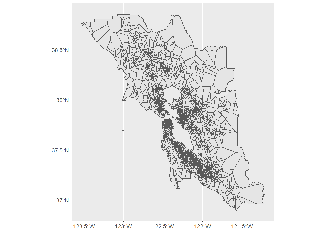
Note that after we get a result out of st_voronoi(), the result is not a normal sf object anymore (rather a more elemental class), so we use st_cast() combined with st_as_sf() to convert it back to our familiar sf class. From there, we use st_intersection() on the st_union() of the Bay Area counties, which essentially cuts the full rectangle-shaped bounds of the voronoi result to just the Bay Area boundary. The last step is to st_join() the object back to the original PurpleAir points so that each voronoi polygon receives the attributes of the original data, most importantly the PM2.5 information.
From here, since we are working with polygons of uniform PM2.5 value, we could use st_intersection() again to cut these voronois by CBGs, similar to our spatial subsetting technique from Section 2.6, and produce weighted averages of PM2.5 for each CBG based on the area of constituent voronoi polygons. We’ll focus on just San Mateo County to reduce the computational complexity of this demonstration.
smc_cbgs <- block_groups("CA","San Mateo", cb = T, progress_bar = F) %>%
  st_transform(4326)

smc_pm25_voronoi_cbg <-
  bay_pm25_voronoi %>%
  st_intersection(smc_cbgs) %>%
  mutate(
    area = st_area(.) %>% as.numeric()
  ) %>%
  group_by(GEOID) %>%
  summarize(
    PM25_week_EPA = weighted.mean(PM25_week_EPA, area, na.rm = T)
  )
Note that the summarize() above, in addition to producing a new PM25_week_EPA result, also merges the associated geometries under the grouping of GEOID, which happens to bring us back to CBG geometries. The weighted.mean() accounts for the relative area of the voronoi polygons subsetted within each CBG.
Let’s map these CBG results, along with the original PurpleAir point sensor data. For the pal, we’ll combine the domains of the original PurpleAir data and the voronoi results, so the minimum and maximum of either are captured in the color range.
smc_list_air <-
  bay_list_air_clean[smc_cbgs, ]

pm25_pal <- colorNumeric(
  palette = "RdYlGn",
  reverse = T,
  domain = c(
    smc_pm25_voronoi_cbg$PM25_week_EPA,
    smc_list_air$PM25_week_EPA
  )
)

leaflet() %>%
  addMapboxTiles(
    style_id = "streets-v11",
    username = "mapbox"
  ) %>%
  addPolygons(
    data = smc_pm25_voronoi_cbg,
    fillColor = ~pm25_pal(PM25_week_EPA),
    fillOpacity = 0.5,
    color = "white",
    weight = 0.5,
    label = ~PM25_week_EPA,
    highlightOptions = highlightOptions(
      weight = 2,
      opacity = 1
    )
  ) %>%
  addCircleMarkers(
    data = smc_list_air,
    fillColor = ~pm25_pal(PM25_week_EPA),
    fillOpacity = 1,
    color = "black",
    weight = 0.5,
    radius = 5,
    label = ~PM25_week_EPA
  ) %>%
  addLegend(
    data = smc_list_air,
    pal = pm25_pal,
    values = ~PM25_week_EPA
  )
Let’s demonstrate one other interpolation technique which may be more realistic than the voronoi polygons (which suggest abrupt discontinuous jumps in PM2.5 right at the boundaries). We would expect air pollution dissipation to be inversely related to distance, i.e. the farther one is away from a pollution source, the less one is expected to be exposed to it. The gstat package can work with geospatial data like our PurpleAir points and create what is equivalent to a 2-dimensional regression affected by the x-y locations and values of all points, with inverse distance weighting. In the following gstat() function, which has a similar structure to lm() from Chapters 3 and 4, a formula of structure PM25_week_EPA ~ 1 has no “independent variable” on the right-hand side of the ~, so the spatial interpolation being performed is only based on PM25_week_EPA values of our existing points, and their x-y locations.
spatial_model is complex mathematically, but intuitively you can imagine it as being able to best predict the PM2.5 value at a new lat/long location, based on the proximity of all other existing PurpleAir sensors. Let’s go ahead and create predictions for all points in the SMC region, but we’ll need to work with rasters, which are essentially pixelated geospatial information. So far, we’ve worked with “vector-based” geometries, which have clear boundaries with distinct shapes, whereas raster information has a boundary dimension and pixel resolution, with all information being contained pixel-by-pixel. We can convert vectors into rasters (imagine saving a file as a JPG and the result becoming pixelated) using st_rasterize() from the stars package (which provides useful functionality on top of the more fundamental raster package). We’ll need to create a rasterized version of the SMC county region to be able to receive spatial interpolation predictions of the same region. st_rasterize() will pick its own resolution by default, but you can specify your own as arguments.
smc_raster <-
  counties("CA", cb = T, progress_bar = F) %>%
  filter(NAME == "San Mateo") %>%
  st_transform(4326) %>%
  st_rasterize()
Typing smc_raster in the console provides summary information about the object, showing in this case that the default process produced a raster with resolution 210 pixels wide by 310 pixels long. Next, let’s use predict() to fill this raster with predicted PM2.5 values.

Now, to distill pixel information back to CBG polygons, we’ll need to conduct some type of summarization of pixel information within the boundary of polygons, which can be done using extract() from the raster package. That function requires both the raster input and the polygon input in more primitive class types than we regularly use (namely stars and sf), so we’ll use as() for quick in-function conversions (into raster and sp types). We’ll also specify our summarization function as mean.
smc_pm25_gstat_cbg <-
  smc_cbgs %>%
  dplyr::select(GEOID) %>%
  mutate(
    PM25_week_EPA = raster::extract(
      as(smc_raster_pm25, "Raster"),
      as(smc_cbgs, "Spatial"),
      fun = mean
    ) %>%
      as.vector()
  )
Note that the result of extract() is not in exactly the form we want, so we need to convert using as.vector() to a pure vector that mutate() is looking for. Also note that both select() and extract() are now ambiguous because we have both tidyverse and raster packages loaded; turns out that these two separate packages did not coordinate well and have lots of duplicately named functions, so we have to be explicit about using dplyr::select() and raster::extract().
The plot below shows the % difference between the gstat and voronoi approaches:
smc_pm25_diff_cbg <-
  smc_pm25_voronoi_cbg %>%
  rename(voronoi_pm25 = PM25_week_EPA) %>%
  left_join(
    smc_pm25_gstat_cbg %>%
      dplyr::select(
        GEOID,
        gstat_pm25 = PM25_week_EPA
      ) %>%
      st_set_geometry(NULL)
  ) %>%
  mutate(
    diff_pm25 = (gstat_pm25 - voronoi_pm25)/gstat_pm25
  )

pm25_diff_pal <- colorNumeric(
  palette = "RdYlGn",
  domain = smc_pm25_diff_cbg$diff_pm25
)

leaflet() %>%
  addMapboxTiles(
    style_id = "streets-v11",
    username = "mapbox"
  ) %>%
  addPolygons(
    data = smc_pm25_diff_cbg,
    fillColor = ~pm25_diff_pal(diff_pm25),
    fillOpacity = 0.5,
    color = "white",
    weight = 0.5,
    label = ~diff_pm25,
    highlightOptions = highlightOptions(
      weight = 2,
      opacity = 1
    )
  ) %>%
  addLegend(
    data = smc_pm25_diff_cbg,
    pal = pm25_diff_pal,
    values = ~diff_pm25,
    title = "(gstat-voronoi)/<br>gstat"
  )
For many CBGs, the difference between the two spatial interpolation approaches is negligible, but for others the difference can be over 50% in one direction or another. For pollution flows like air and water, I would recommend the inverse distance weighting approach over Voronoi polygons, but there is a yet more sophisticated approach called “Kriging” which is beyond the scope of this chapter, but builds off the gstat spatial interpolation function with even more rigorous statistical modeling (one key flaw with the current inverse distancing weighting approach is that it is treating each existing PurpleAir sensor as an emissions source, so fails to capture certain broader trends of air pollution passing through a region).
To conclude this section, we’ll show how to retrieve data further back in time from PurpleAir. If you want to conduct more detailed longitudinal analysis, or produce averages over a longer timescale than just the past week, then the standard dataset we’ve used so far won’t be adequate. purpleairDownload() allows you to specify, for a subset of sensors, a start date and end date of data from 10 minute intervals up to daily intervals, and receive all possible data retrievable from PurpleAir. This would take a while to do for all sensors in the Bay Area, so I’d recommend focusing your inquiry. In the example below, I take just two sensors that are on Stanford campus (feel free to look for them on the PurpleAir site yourself), one outdoor and one indoor, and download daily data from September and October 2020 (during which time there were some wildfires nearby).
(Note that this function may require a special version of a package doMC to be installed, so we’re doing a special version of install.packages() in the chunk below.)
install.packages("doMC", repos="http://R-Forge.R-project.org")

sensors <- bay_list_air %>%
  filter(Label %in% c("RH1- Stanford Law School","Olmsted Road")) %>%
  st_set_geometry(NULL)

temp <- tempfile()

purpleairDownload(
  site.csv = sensors,
    start.date = "2020-9-24",
    end.date = "2020-10-31",
    output.path = temp,
    average = 1440,
    time.zone = 'America/Los_Angeles'
)

airdata <-
  sensors$ID %>%
  map_dfr(
    ~ read_csv(
      paste0(temp,"/",.,".csv")
    )
  )

unlink(temp)
average= can be modified to be various options from 10 (10 minutes) to 1440 (a full day). The map_dfr() incorporates some shorthand given how minimal of a looping execution is required, reading CSVs that have been created by purpleairDownload() in the temp location. Let’s do a little bit of data cleaning, and then plot our results:
airdata_clean <-
  airdata %>%
  transmute(
    Location = Location,
    PM2.5 = 0.534*`PM2.5_CF_1_ug/m3_A` - 0.0844*`Humidity_%_A` + 5.604,
    date =
      substr(created_at, 1, 10) %>% as.Date()
  )

airdata_clean %>%
  ggplot() +
  geom_line(
    aes(
      x = date,
      y = PM2.5,
      color = Location
    )
  )
If one were to gather a larger sample of indoor vs. outdoor sensors in the Bay Area, one would expect to find a similar noticeable gap in air quality during major wildfire events, a subject which will be further considered in Chapter 8.