4.2 Building emissions

We have already introduced energy data in the intro textbook and parcel data in Section 2.2. In the absence of direct building-level energy data, aggregated energy data can still be used to estimate GHG emissions from building energy use for large regions, and can be combined with aggregated parcel data to gain insights about energy efficiency.

Let’s start by reading 2021 PG&E electricity and gas data. We can use the same technique as we used before, but this time make use of an additional nested for loop to loop through both “Electric” and “Gas” files from the PG&E site. We need to deal with differences in the field names of each kind of CSV, where electricity data is provided as TOTALKWH (kilowatt-hours) while gas data is provided as TOTALTHM (therms). To deal with these different units, and since we ultimately want to get to GHG emissions in units of metric tonnes of carbon equivalent, we can convert both fields to TOTALTCO2E within the loop before binding the different quarterly files together.

Converting from electricity or gas units to CO2 equivalent depends on some knowledge of the actual technological operations involved. Starting with electricity, which can have highly variable emissions depending on the generation sources, we can use PG&E’s voluntary emissions reporting which can be viewed at their Corporate Sustainability page under “Benchmarking Greenhouse Gas Emissions for Delivered Electricity”. Plotting the table information yields the following:

library(tigris)
library(tidyverse)
library(sf)
library(leaflet)
library(mapboxapi)

pge_elec_emissions_factor <-
  data.frame(
    year = c(2013:2019),
    factor = c(427,435,405,294,210,206,2.68)
  )

pge_elec_emissions_factor %>% 
  ggplot() +
  geom_line(
    aes(
      x = year,
      y = factor
    )
  ) +
  labs(
    x = "Year",
    y = "Pounds of CO2 per MHh",
    title = "PG&E electricity emissions rate"
  )

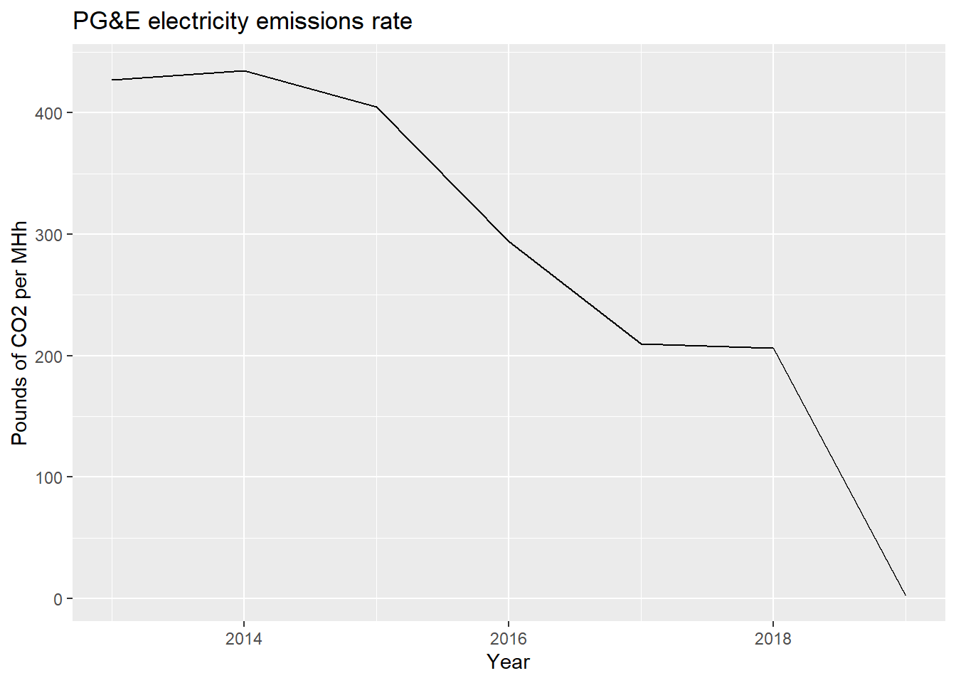
With these factors, we can convert kWh to MWh to pounds of CO2, and from there, to metric tonnes (1 pound = 0.000453592 metric tonnes, according to Google).

Keep in mind that in the Bay Area, many community choice aggregators, such as CleanPowerSF in San Francisco, provide an alternative electricity generation option for consumers with increased renewable energy content, potentially up to zero carbon emissions (PG&E is still responsible for delivery through its wires and infrastructure). This demonstration will assume that the PG&E data shows full electricity consumption including CCA-generated electricity, and accounts for that portion of electricity usage having a lower carbon footprint.

For natural gas, since the composition of PG&E’s natural gas does not change significantly over time, we’ll use just one emissions factor from the U.S. Energy Information Administration, which is 117 pounds of CO2 per million BTU. So we can convert therms to MBTUs to pounds of CO2, and from there, to metric tonnes; the conversion ends up being 0.00531 metric tonnes per therm.

One last note before we process the PG&E data: it turns out that there is an error in 2017 Q4 data downloaded from the website, where Q4 accidentally includes September 2017, which should only be part of Q3. This is the kind of data issue that one should always be on the lookout for when working with new datasets. We’ll remove that double-counted September 2017 data manually.

pge_data <- 
  2013:2019 %>% 
  map_dfr(function(yr){
    
    factor <- 
      pge_elec_emissions_factor %>% 
      filter(year == yr) %>% 
      pull(factor)
    
    1:4 %>% 
      map_dfr(function(quarter){
        
        c("Electric","Gas") %>% 
          map_dfr(function(type){
            
            filename <- 
              paste0(
                "pge/PGE_",
                yr,
                "_Q",
                quarter,
                "_",
                type,
                "UsageByZip.csv"
              )
            
            temp <- read_csv(filename)
            
            if(yr == 2017 & quarter == 4) {
              temp <- 
                temp %>% 
                filter(MONTH != 9)
            }
            
            temp <-
              temp %>% 
              rename_all(toupper) %>% 
              mutate(
                TOTALKBTU = ifelse(
                  substr(CUSTOMERCLASS,1,1) == "E",
                  TOTALKWH * 3.412,
                  TOTALTHM * 99.976
                ),
                TOTALTCO2E = ifelse(
                  substr(CUSTOMERCLASS,1,1) == "E",
                  TOTALKWH/1000 * factor * 0.000453592,
                  TOTALTHM * 0.00531
                )
              ) %>% 
              select(
                ZIPCODE,
                YEAR,
                MONTH,
                CUSTOMERCLASS,
                TOTALKBTU,
                TOTALTCO2E,
                TOTALCUSTOMERS
              )
            
          })
        
      })
    
  })

Now, let’s filter to just ZIP codes in San Francisco, filter to just residential and commercial electricity (given that industrial sources will tend to be masked in the public PG&E data due to the CPUC 15-15 rule, which limits utility companies from sharing data that is too individualized) and plot the change in KBTU and TCO2E over the years.

us_zips <- 
  zctas(cb = T, progress_bar = F)

sf_zips <- 
  us_zips %>% 
  st_centroid() %>% 
  .[counties("CA", cb = T, progress_bar = F) %>% filter(NAME == "San Francisco"), ] %>% 
  st_drop_geometry() %>% 
  left_join(us_zips %>% select(GEOID10)) %>% 
  st_as_sf() %>% 
  st_transform(4326)

sf_pge_data <-
  pge_data %>% 
  filter(ZIPCODE %in% sf_zips$ZCTA5CE10) %>% 
  filter(CUSTOMERCLASS %in% c(
    "Elec- Commercial",
    "Elec- Residential",
    "Gas- Commercial",
    "Gas- Residential"
  )) %>% 
  mutate(
    ENERGYTYPE = substr(CUSTOMERCLASS,1,1)
  ) %>% 
  group_by(ZIPCODE, ENERGYTYPE, YEAR) %>% 
  summarize(
    TOTALKBTU = sum(TOTALKBTU, na.rm=T),
    TOTALTCO2E = sum(TOTALTCO2E, na.rm=T), 
    TOTALCUSTOMERS = mean(TOTALCUSTOMERS, na.rm=T)
  ) %>% 
  group_by(ENERGYTYPE, YEAR) %>%
  summarize(across(
    c(TOTALKBTU,TOTALTCO2E,TOTALCUSTOMERS),
    ~sum(.,na.rm=T)
  ))

Note that we group_by() two times here. The first time, we are collapsing the data by month. When combining monthly energy usage to annual totals, sum() is correct, but when combining monthly customers to annual totals, since the customer base is likely to be mostly the same from month to month, mean() is likely to be a more accurate estimate. Then, for the second group_by(), we collapse by ZIP code, in which case summing on all three variables is correct.

ggplot(
  sf_pge_data, 
  aes(
    x = as.factor(YEAR), 
    y = TOTALKBTU/1000000
  )
) + 
  geom_bar(stat = "identity", aes(fill = ENERGYTYPE), position = "dodge") + 
  labs(x = "Year", y = "GBTU", title = "SF Annual Energy Usage, 2013 to 2019") + 
  scale_fill_discrete(name="Energy Type",labels = c("Electricity","Gas"))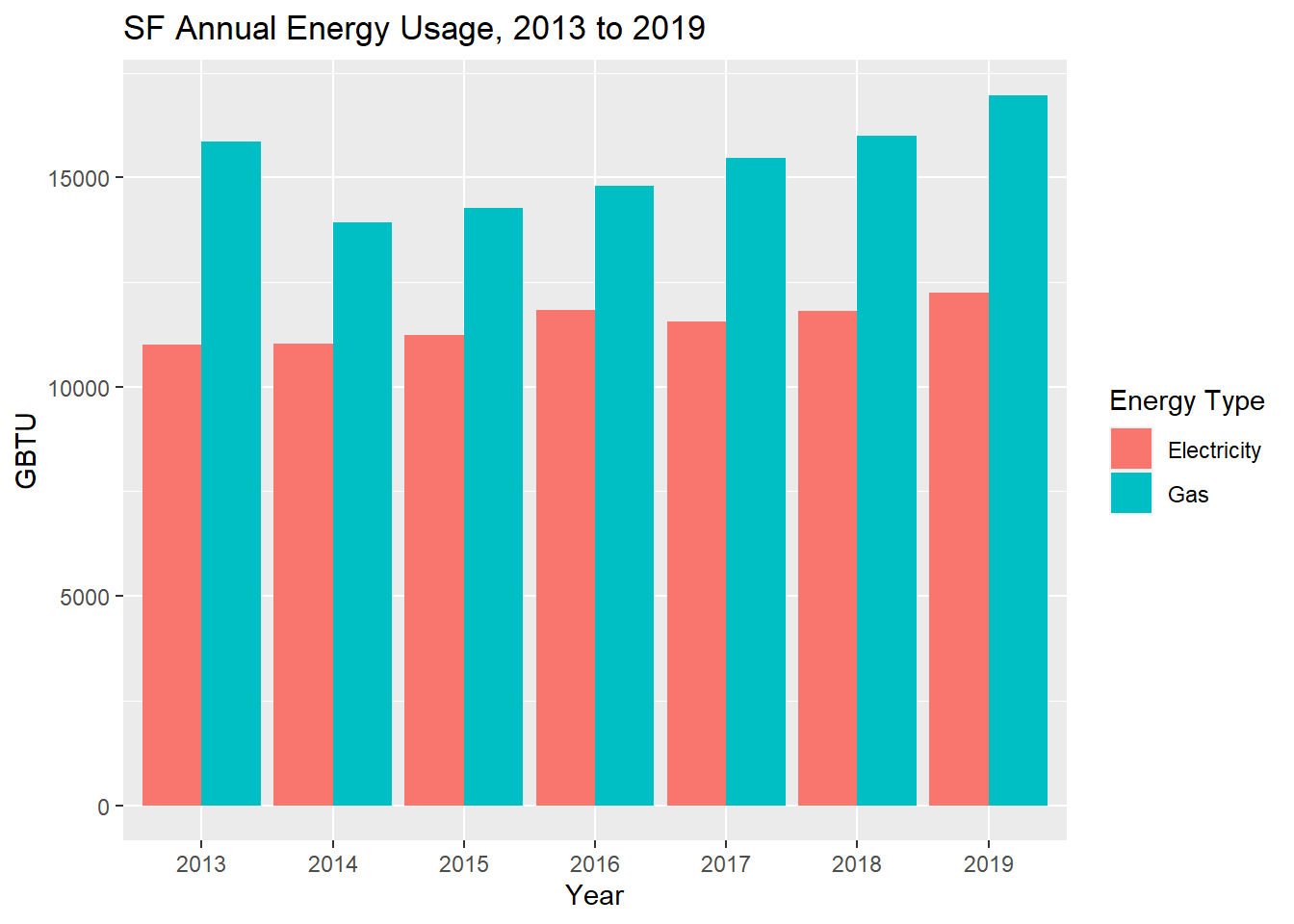

ggplot(
  sf_pge_data, 
  aes(
    x = as.factor(YEAR), 
    y = TOTALTCO2E
  )
) + 
  geom_bar(stat = "identity", aes(fill = ENERGYTYPE), position = "dodge") + 
  labs(x = "Year", y = "tCO2e", title = "SF Annual Energy Usage, 2013 to 2019") + 
  scale_fill_discrete(name="Energy Type",labels = c("Electricity","Gas"))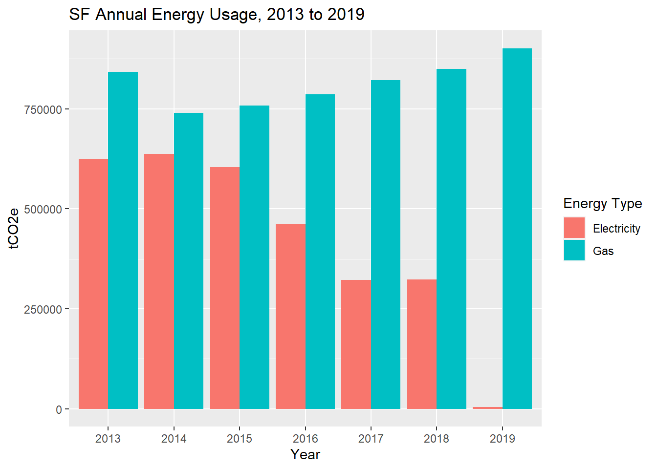

The sharp divergence in carbon footprint between gas and electricity use, given the increasing renewable content in electricity generation, is a key reason why cities are pushing for building electrification as a key GHG mitigation approach.

Besides tracking total emissions, it is still important to focus on measures of energy use intensity (energy use per square foot), since this may be a key lever point for reducing building emissions further (besides reducing the carbon content of the energy source itself). To do that involves revisiting parcel data as we explored in Section 2.2, which would allow us to calculate the total amount of building square footage at the same scale as our energy data. Let’s return to the SF Assessor-Recorder website, and since we are working with energy data from 2013 to 2019, we can try to match parcel data year by year. Below, you can see the same approach applied multiple times to read different years of data. We generally assume the data dictionary and use codes will be the same, but this is the kind of scale of analysis where things can get messy, so it is worth it to check each dataset carefully (e.g., reviewing each year’s data dictionary and use code supplementary sheet tabs, which I’m not showing in detail below). The one obvious inconsistency at initial reading is that the 2014-2015 dataset is named differently and doesn’t seem to include a data dictionary.

temp <- tempfile()
download.file("https://sfassessor.org/sites/default/files/uploaded/2019.8.20__SF_ASR_Secured_Roll_Data_2012-2013.xlsx",destfile = temp, mode = "wb")
sf_secured_13 <- read_excel(temp, sheet = "Roll Data 2012-2013")
saveRDS(sf_secured_13, "sf_secured_13.rds")
unlink(temp)

temp <- tempfile()
download.file("https://sfassessor.org/sites/default/files/uploaded/2019.8.20__SF_ASR_Secured_Roll_Data_2013-2014.xlsx",destfile = temp, mode = "wb")
sf_secured_14 <- read_excel(temp, sheet = "Roll Data 2013-2014")
saveRDS(sf_secured_14, "sf_secured_14.rds")
unlink(temp)

temp <- tempfile()
download.file("https://sfassessor.org/sites/default/files/uploaded/2019.8.20__SF_ASR_Secured_Roll_Data_2014-2015.xlsx",destfile = temp, mode = "wb")
sf_secured_15 <- read_excel(temp, sheet = "2014-2015")
saveRDS(sf_secured_15, "sf_secured_15.rds")
unlink(temp)

temp <- tempfile()
download.file("https://sfassessor.org/sites/default/files/uploaded/2020.7.10_SF_ASR_Secured_Roll_Data_2015-2016.xlsx",destfile = temp, mode = "wb")
sf_secured_16 <- read_excel(temp, sheet = "Roll Data 2015-2016")
saveRDS(sf_secured_16, "sf_secured_16.rds")
unlink(temp)

temp <- tempfile()
download.file("https://sfassessor.org/sites/default/files/uploaded/2019.8.12__SF_ASR_Secured_Roll_Data_2016-2017_0.xlsx",destfile = temp, mode = "wb")
sf_secured_17 <- read_excel(temp, sheet = "Roll Data 2016-2017")
saveRDS(sf_secured_17, "sf_secured_17.rds")
unlink(temp)

temp <- tempfile()
download.file("https://sfassessor.org/sites/default/files/uploaded/2019.8.12__SF_ASR_Secured_Roll_Data_2017-2018_0.xlsx",destfile = temp, mode = "wb")
sf_secured_18 <- read_excel(temp, sheet = "Roll Data 2017-2018")
saveRDS(sf_secured_18, "sf_secured_18.rds")
unlink(temp)

temp <- tempfile()
download.file("https://sfassessor.org/sites/default/files/uploaded/2020.7.10_SF_ASR_Secured_Roll_Data_2018-2019.xlsx",destfile = temp, mode = "wb")
sf_secured_19 <- read_excel(temp, sheet = "Roll Data 2018-2019")
saveRDS(sf_secured_19, "sf_secured_19.rds")
unlink(temp)

Note that I use saveRDS() to save each file right after creating. The benefit of saveRDS() paired with readRDS() will be the freedom to perform looped operations more easily on these locally stored files, as I’ll show soon.

Since our focus here is narrowly on residential and commercial building square footage ZIP code, we can ignore much of the complexity of these datasets and focus on:

• Identifying the location of each parcel (expecting some unsuccessful joins here and there) so that we can spatial join them to ZIP codes.
• Filtering to just the residential and commercial uses, which requires determining which use codes in RP1CLACDE are residential vs. commercial vs. other. One challenge will be separating out mixed use buildings, which, for simplicity, we’ll treat as their own third group and then divide their aggregate square footage equally between residential and commercial.
• Grouping and summarizing square footage, SQFT, which, by the way, is described in the data dictionaries as “Property Area in Square Feet - Same as lot area”, but, upon inspection, is clearly not the same as the other field “Lot Area”.

sf_parcels_shape <- 
  st_read("https://data.sfgov.org/api/geospatial/acdm-wktn?method=export&format=GeoJSON") %>% 
  select(apn = blklot)

We will use a for loop with our looping variable being the year portion of the file name, which will allow us to easily read the data we just stored into a dummy variable named data:

sf_secured_summary <- 13:19 %>% 
  map_dfr(function(year){
  
    readRDS(paste0("sf_secured_", year, ".rds")) %>% 
      mutate(
        apn = RP1PRCLID %>% 
          str_replace(" ","")
      ) %>% 
      left_join(sf_parcels_shape) %>% 
      st_as_sf() %>% 
      st_centroid() %>% 
      st_join(
        sf_zips %>% 
          select(ZIPCODE = GEOID10)
      ) %>% 
      st_drop_geometry() %>% 
      mutate(
        TYPE = case_when(
          RP1CLACDE %in% c("A","A15","A5","CO","COS","D","DA","DA15","DA5","DBM","DCON","DD","DD15","DD5","DF","F","F15","F5","FA","FA15","FA5","LZ","LZBM","N2","RH","TH","THBM","TI15","TIA","TIC","TIC5","TIF","TS","TSF","TSU","XV","Z","ZBM") ~ "Residential",
          RP1CLACDE %in% c("AC","F2","FS","FS15","FS5","MIX","OA","OA15","OA5") ~ "Mixed",
          !RP1CLACDE %in% c("I","IDC","IW","IX","IZ") ~ "Commercial"
        )
      ) %>% 
      filter(!is.na(TYPE)) %>% 
      group_by(ZIPCODE, TYPE) %>% 
      summarize(SQFT = sum(SQFT, na.rm = T)) %>% 
      pivot_wider(
        names_from = TYPE,
        values_from = SQFT
      ) %>% 
      mutate(
        Commercial = Commercial + Mixed/2,
        Residential = Residential + Mixed/2
      ) %>% 
      select(-Mixed) %>% 
      filter(!is.na(Commercial) & !is.na(Residential)) %>% 
      pivot_longer(
        -ZIPCODE,
        names_to = "TYPE",
        values_to = "SQFT"
      ) %>% 
      mutate(YEAR = paste0(20,year) %>% as.numeric())
})

Let’s plot building square footage over time, separated between commercial and residential:

sf_secured_summary %>% 
  group_by(YEAR, TYPE) %>% 
  summarize(SQFT = sum(SQFT)) %>% 
  ggplot(
    aes(
      x = as.factor(YEAR), 
      y = SQFT/1000000
    )
  ) + 
  geom_bar(stat = "identity", aes(fill = TYPE), position = "dodge") + 
  labs(x = "Year", y = "Square Footage, Millions", title = "SF Annual Building Square Footage, 2013 to 2019") + 
  scale_fill_discrete(name="Type")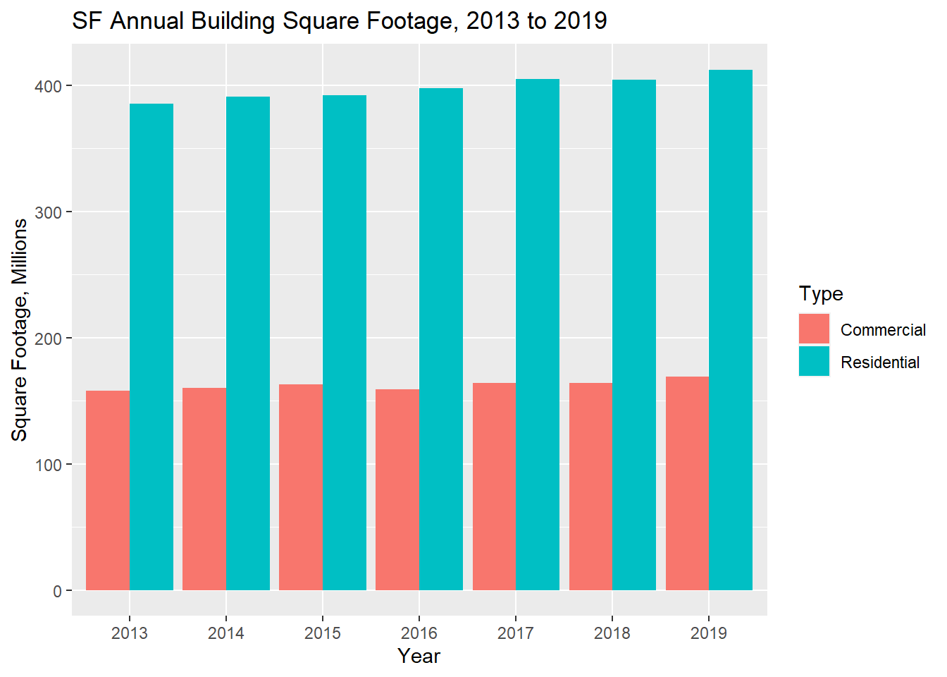

And now, let’s merge the two datasets together and plot energy use intensity, separated by commercial vs. residential as well as electricity vs. gas. In this case, using geom_line() will make for clearer viewing:

sf_pge_sqft <-
  pge_data %>% 
  filter(ZIPCODE %in% sf_secured_summary$ZIPCODE) %>% 
  filter(CUSTOMERCLASS %in% c(
    "Elec- Commercial",
    "Elec- Residential",
    "Gas- Commercial",
    "Gas- Residential"
  )) %>% 
  mutate(
    ZIPCODE = ZIPCODE %>% as.character(),
    ENERGYTYPE = substr(CUSTOMERCLASS,1,1),
    TYPE = substr(CUSTOMERCLASS,6,nchar(CUSTOMERCLASS)) %>% str_trim()
  ) %>% 
  group_by(ZIPCODE, ENERGYTYPE, TYPE, YEAR) %>% 
  summarize(
    TOTALKBTU = sum(TOTALKBTU, na.rm=T)
  ) %>% 
  left_join(
    sf_secured_summary,
    by = c("ZIPCODE","YEAR","TYPE")
  ) %>% 
  filter(!is.na(SQFT)) %>% 
  mutate(
    KBTU_SQFT = TOTALKBTU/SQFT
  )

sf_pge_sqft %>% 
  group_by(YEAR, ENERGYTYPE, TYPE) %>% 
  summarize(
    TOTALKBTU = sum(TOTALKBTU),
    SQFT = sum(SQFT)
  ) %>% 
  mutate(
    KBTU_SQFT = TOTALKBTU/SQFT
  ) %>% 
  ggplot(
    aes(
      x = YEAR,
      y = KBTU_SQFT
    )
  ) + 
  geom_line(
    aes(
      color = TYPE,
      linetype = ENERGYTYPE
    ),
    size = 1
  ) +
  labs(x = "Year", y = "kBTUs per Sqft", title = "SF Annual Building Energy Use Intensity, 2013 to 2019", color ="Use Type", linetype = "Energy Type") +
  scale_linetype_manual(values = c("solid","dotted"), labels = c("Electricity","Gas"))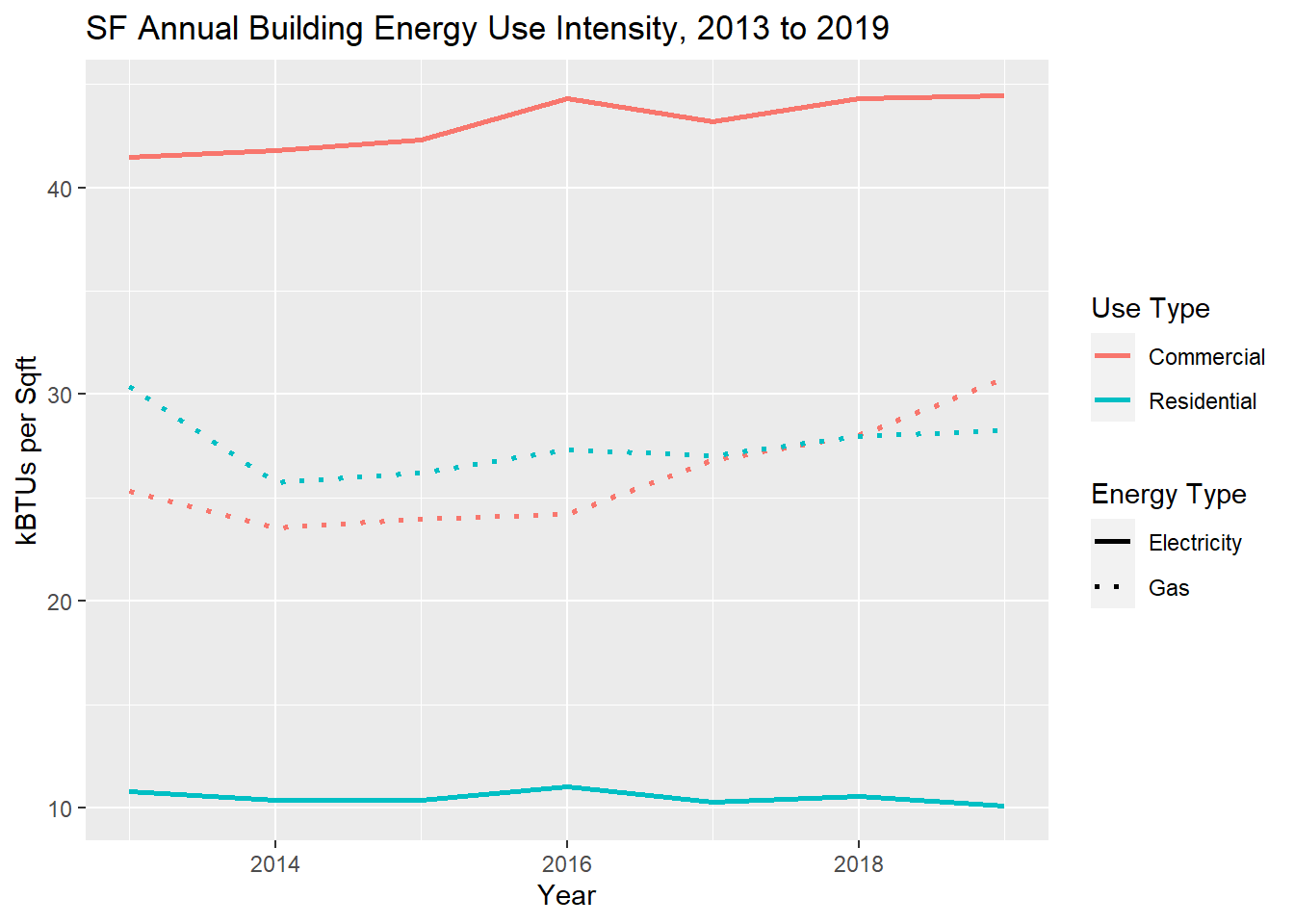

It’s interesting to observe the large divide between electricity use intensity in commercial vs. residential, but pretty similar gas use intensity. One possible interpretation is that, since gas is primarily used for heating, which is not as variable of a demand per square foot, the gas use intensities are more similar, at least relative to electricity use, which could be widely different depending on unique plug loads.

To conclude, let’s map our various results by ZIP code. These chunks are meant to demonstrate how one can quickly visualize many slices of data for potential insights, using mostly copy-and-paste code.

sf_pge_sqft_19 <-
  sf_pge_sqft %>% 
  filter(YEAR == 2019) %>% 
  left_join(sf_zips %>% select(ZIPCODE = GEOID10)) %>% 
  st_as_sf()

pal1 <- colorNumeric(
  palette = "Reds",
  domain = sf_pge_sqft_19 %>% 
    filter(ENERGYTYPE == "E", TYPE == "Commercial") %>% 
    pull(TOTALKBTU)
)

pal2 <- colorNumeric(
  palette = "Blues",
  domain = sf_pge_sqft_19 %>% 
    filter(ENERGYTYPE == "E", TYPE == "Commercial") %>% 
    pull(SQFT)
)

pal3 <- colorNumeric(
  palette = "Purples",
  domain = sf_pge_sqft_19 %>% 
    filter(ENERGYTYPE == "E", TYPE == "Commercial") %>% 
    pull(KBTU_SQFT)
)

sf_pge_sqft_19 %>% 
  filter(ENERGYTYPE == "E", TYPE == "Commercial") %>% 
  leaflet() %>% 
  addMapboxTiles(
    style_id = "streets-v11",
    username = "mapbox"
  ) %>% 
  addPolygons(
    fillColor = ~pal1(TOTALKBTU),
    fillOpacity = 0.5,
    stroke = F,
    label = ~TOTALKBTU %>% signif(2),
    group = "KBTU"
  ) %>% 
  addPolygons(
    fillColor = ~pal2(SQFT),
    fillOpacity = 0.5,
    stroke = F,
    label = ~SQFT %>% signif(2),
    group = "SQFT"
  ) %>% 
  addPolygons(
    fillColor = ~pal3(KBTU_SQFT),
    fillOpacity = 0.5,
    stroke = F,
    label = ~KBTU_SQFT %>% signif(2),
    group = "KBTU/SQFT"
  ) %>% 
  addLegend(
    pal = pal1,
    values = ~TOTALKBTU,
    title = "Total KBTU",
    group = "KBTU"
  ) %>% 
  addLegend(
    pal = pal2,
    values = ~SQFT,
    title = "Total sqft",
    group = "SQFT"
  ) %>% 
  addLegend(
    pal = pal3,
    values = ~KBTU_SQFT,
    title = "KBTU/sqft",
    group = "KBTU/SQFT"
  ) %>% 
  addLayersControl(
    overlayGroups = c("KBTU","SQFT","KBTU/SQFT"),
    position = "bottomright",
    options = layersControlOptions(collapsed = FALSE)
  ) %>% 
  addControl("Commercial Electricity", position = "bottomright") %>% 
  hideGroup("SQFT") %>% 
  hideGroup("KBTU/SQFT")

Note that, currently, only overlayGroups (not baseGroups) allows for legends to be toggled on/off like the layers themselves. This adds the extra step for the user to uncheck/check each desired layer. The baseGroups version can be made to work in a Shiny dashboard.

pal1 <- colorNumeric(
  palette = "Reds",
  domain = sf_pge_sqft_19 %>% 
    filter(ENERGYTYPE == "G", TYPE == "Commercial") %>% 
    pull(TOTALKBTU)
)

pal2 <- colorNumeric(
  palette = "Blues",
  domain = sf_pge_sqft_19 %>% 
    filter(ENERGYTYPE == "G", TYPE == "Commercial") %>% 
    pull(SQFT)
)

pal3 <- colorNumeric(
  palette = "Purples",
  domain = sf_pge_sqft_19 %>% 
    filter(ENERGYTYPE == "G", TYPE == "Commercial") %>% 
    pull(KBTU_SQFT)
)

sf_pge_sqft_19 %>% 
  filter(ENERGYTYPE == "G", TYPE == "Commercial") %>% 
  leaflet() %>% 
  addMapboxTiles(
    style_id = "streets-v11",
    username = "mapbox"
  ) %>% 
  addPolygons(
    fillColor = ~pal1(TOTALKBTU),
    fillOpacity = 0.5,
    stroke = F,
    label = ~TOTALKBTU %>% signif(2),
    group = "KBTU"
  ) %>% 
  addPolygons(
    fillColor = ~pal2(SQFT),
    fillOpacity = 0.5,
    stroke = F,
    label = ~SQFT %>% signif(2),
    group = "SQFT"
  ) %>% 
  addPolygons(
    fillColor = ~pal3(KBTU_SQFT),
    fillOpacity = 0.5,
    stroke = F,
    label = ~KBTU_SQFT %>% signif(2),
    group = "KBTU/SQFT"
  ) %>% 
  addLegend(
    pal = pal1,
    values = ~TOTALKBTU,
    title = "Total KBTU",
    group = "KBTU"
  ) %>% 
  addLegend(
    pal = pal2,
    values = ~SQFT,
    title = "Total sqft",
    group = "SQFT"
  ) %>% 
  addLegend(
    pal = pal3,
    values = ~KBTU_SQFT,
    title = "KBTU/sqft",
    group = "KBTU/SQFT"
  ) %>% 
  addLayersControl(
    overlayGroups = c("KBTU","SQFT","KBTU/SQFT"),
    position = "bottomright",
    options = layersControlOptions(collapsed = FALSE)
  ) %>% 
  addControl("Commercial Gas", position = "bottomright") %>% 
  hideGroup("SQFT") %>% 
  hideGroup("KBTU/SQFT")

pal1 <- colorNumeric(
  palette = "Reds",
  domain = sf_pge_sqft_19 %>% 
    filter(ENERGYTYPE == "E", TYPE == "Residential") %>% 
    pull(TOTALKBTU)
)

pal2 <- colorNumeric(
  palette = "Blues",
  domain = sf_pge_sqft_19 %>% 
    filter(ENERGYTYPE == "E", TYPE == "Residential") %>% 
    pull(SQFT)
)

pal3 <- colorNumeric(
  palette = "Purples",
  domain = sf_pge_sqft_19 %>% 
    filter(ENERGYTYPE == "E", TYPE == "Residential") %>% 
    pull(KBTU_SQFT)
)

sf_pge_sqft_19 %>% 
  filter(ENERGYTYPE == "E", TYPE == "Residential") %>% 
  leaflet() %>% 
  addMapboxTiles(
    style_id = "streets-v11",
    username = "mapbox"
  ) %>% 
  addPolygons(
    fillColor = ~pal1(TOTALKBTU),
    fillOpacity = 0.5,
    stroke = F,
    label = ~TOTALKBTU %>% signif(2),
    group = "KBTU"
  ) %>% 
  addPolygons(
    fillColor = ~pal2(SQFT),
    fillOpacity = 0.5,
    stroke = F,
    label = ~SQFT %>% signif(2),
    group = "SQFT"
  ) %>% 
  addPolygons(
    fillColor = ~pal3(KBTU_SQFT),
    fillOpacity = 0.5,
    stroke = F,
    label = ~KBTU_SQFT %>% signif(2),
    group = "KBTU/SQFT"
  ) %>% 
  addLegend(
    pal = pal1,
    values = ~TOTALKBTU,
    title = "Total KBTU",
    group = "KBTU"
  ) %>% 
  addLegend(
    pal = pal2,
    values = ~SQFT,
    title = "Total sqft",
    group = "SQFT"
  ) %>% 
  addLegend(
    pal = pal3,
    values = ~KBTU_SQFT,
    title = "KBTU/sqft",
    group = "KBTU/SQFT"
  ) %>% 
  addLayersControl(
    overlayGroups = c("KBTU","SQFT","KBTU/SQFT"),
    position = "bottomright",
    options = layersControlOptions(collapsed = FALSE)
  ) %>% 
  addControl("Residential Electricity", position = "bottomright") %>% 
  hideGroup("SQFT") %>% 
  hideGroup("KBTU/SQFT")

pal1 <- colorNumeric(
  palette = "Reds",
  domain = sf_pge_sqft_19 %>% 
    filter(ENERGYTYPE == "G", TYPE == "Residential") %>% 
    pull(TOTALKBTU)
)

pal2 <- colorNumeric(
  palette = "Blues",
  domain = sf_pge_sqft_19 %>% 
    filter(ENERGYTYPE == "G", TYPE == "Residential") %>% 
    pull(SQFT)
)

pal3 <- colorNumeric(
  palette = "Purples",
  domain = sf_pge_sqft_19 %>% 
    filter(ENERGYTYPE == "G", TYPE == "Residential") %>% 
    pull(KBTU_SQFT)
)

sf_pge_sqft_19 %>% 
  filter(ENERGYTYPE == "G", TYPE == "Residential") %>% 
  leaflet() %>% 
  addMapboxTiles(
    style_id = "streets-v11",
    username = "mapbox"
  ) %>% 
  addPolygons(
    fillColor = ~pal1(TOTALKBTU),
    fillOpacity = 0.5,
    stroke = F,
    label = ~TOTALKBTU %>% signif(2),
    group = "KBTU"
  ) %>% 
  addPolygons(
    fillColor = ~pal2(SQFT),
    fillOpacity = 0.5,
    stroke = F,
    label = ~SQFT %>% signif(2),
    group = "SQFT"
  ) %>% 
  addPolygons(
    fillColor = ~pal3(KBTU_SQFT),
    fillOpacity = 0.5,
    stroke = F,
    label = ~KBTU_SQFT %>% signif(2),
    group = "KBTU/SQFT"
  ) %>% 
  addLegend(
    pal = pal1,
    values = ~TOTALKBTU,
    title = "Total KBTU",
    group = "KBTU"
  ) %>% 
  addLegend(
    pal = pal2,
    values = ~SQFT,
    title = "Total sqft",
    group = "SQFT"
  ) %>% 
  addLegend(
    pal = pal3,
    values = ~KBTU_SQFT,
    title = "KBTU/sqft",
    group = "KBTU/SQFT"
  ) %>% 
  addLayersControl(
    overlayGroups = c("KBTU","SQFT","KBTU/SQFT"),
    position = "bottomright",
    options = layersControlOptions(collapsed = FALSE)
  ) %>% 
  addControl("Residential Gas", position = "bottomright") %>% 
  hideGroup("SQFT") %>% 
  hideGroup("KBTU/SQFT")

Other notable ways to think about building energy use include dividing energy use per capita instead of per sqft, which would imply processing census data about residential and commercial occupants of buildings, or dividing energy use by heating and cooling degree days, which are measures of how many “degrees of temperature difference” between outdoor air and indoor thermostat preferences there were throughout an entire year (some quantity that needed to be overcome by heating and some amount by cooling, respectively). Each of these dimensions (building size, building occupancy, and climate), and many others, interact in nontrivial ways to impact building energy use and emissions.