2.1 Geospatial data

The heart of urban data analytics is spatial data. We will consider geospatial techniques, along with an understanding of U.S. geographies, as central to understanding how to use R for urban problem solving in a U.S. context.

sf is the standard package and geospatial object type nowadays for any geospatial work in R, and you can find the best overview here. For our purposes, I’ll start by demonstrating how to bring in Census geographies using tigris, which is a package that is designed to make it easy to pull data from the U.S. Census Bureau’s TIGER database (think back to the section on reading files, Option 4, and imagine this to be a set of convenient functions that simplify steps you could otherwise figure out manually yourself).

tigris has a variety of functions, but the most common ones you’ll use throughout this curriculum have intuitive names to grab the most common Census geographies: counties(), tracts(),block_groups(), and blocks(). Each one has slightly different arguments you need to provide. Here’s an example grabbing all counties in California:

library(tidyverse)
library(sf)
library(tigris)
library(mapview)
library(leaflet)

ca_counties <- counties("CA", cb = T, progress_bar = F)

For counties(), you need to supply a state and can only receive a full set of counties for a state at a time. cb = T gives you simplified geometries but they are roughly clipped to the shoreline; cb = F gives you the most detailed geometries available, but geometries with coastlines may have strange water portions included; for the improved visualization I’d generally recommend cb = T. progress_bar = F only matters for knitting to a web page; it prevents a lot of unnecessary progress outputs from being displayed, which the standard knitr options can’t prevent. tigris automatically creates outputs that are sf objects (one of a few possible formats for geospatial data), which you can confirm by running class(ca_counties) in the Console.

It’s important in geospatial work to know your coordinate reference system. Here’s how to check for a geospatial object:

st_crs(ca_counties)

## Coordinate Reference System:
##   User input: NAD83 
##   wkt:
## GEOGCRS["NAD83",
##     DATUM["North American Datum 1983",
##         ELLIPSOID["GRS 1980",6378137,298.257222101,
##             LENGTHUNIT["metre",1]]],
##     PRIMEM["Greenwich",0,
##         ANGLEUNIT["degree",0.0174532925199433]],
##     CS[ellipsoidal,2],
##         AXIS["latitude",north,
##             ORDER[1],
##             ANGLEUNIT["degree",0.0174532925199433]],
##         AXIS["longitude",east,
##             ORDER[2],
##             ANGLEUNIT["degree",0.0174532925199433]],
##     ID["EPSG",4269]]

A lot of information is provided, but what is most salient here should be that the EPSG is 4269, which refers to this standard classification system. I won’t explain geography concepts here in detail (this video may help), but just note that when joining two sf objects you need matching coordinate reference systems, and these EPSG codes are recognized by sf as input options. tigris data is always in 4269. You can transform using st_transform(). Google Maps coordinates are in EPSG:4326, which is effectively the same as 4269. Geospatial operations in planar geometry (like buffering) need to happen in a projected coordinate system, and I typically use EPSG:26910 for that, or my own custom version that measures in feet instead of meters, and is written out in a more detailed way using “projection strings” which are yet another standardized formatting option for geographers. The chunk below demonstrates how to go back and forth between all of these.

projection <- "+proj=utm +zone=10 +ellps=GRS80 +datum=NAD83 +units=ft +no_defs"

ca_counties_transformed <- 
  ca_counties %>% 
  st_transform(4326) %>% 
  st_transform(26910) %>% 
  st_transform(projection) %>% 
  st_transform(st_crs(ca_counties))

For the most part, I’d just recommend using whatever consistent EPSG code requires the least manual transforming for a specific code document, but a more universal strategy would be to instantiate projection in your initial setup chunk and then always st_transform(projection). However, note that the leaflet() mapping function, which we’ll encounter soon, prefers certain ESPGs (like 4326 or 4269), so I’ll usually just do one last conversion of everything back to 4326 or 4269, as necessary, after I’ve completed all my geospatial analyses (these would be an ideal universal CRS, but you can’t do the various planar operations in them).

The fastest way to map is using ggplot() + geom_sf() on individual sf objects which gives you a fixed map in your File window. Another popular option is mapview() in the mapview package, which can create an interactive map with some preset visual choices (I prefer this for a quick visualization in the Console). But for any mapping for formal communication of your work, I recommend interactive maps with the fully customizable leaflet(), with a comprehensive overview here. Multiple approaches are demonstrated below.

ggplot(ca_counties) + geom_sf()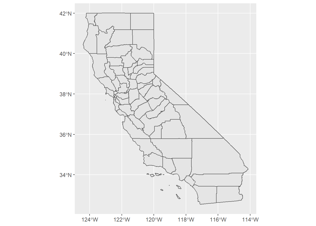

mapview(ca_counties)

leaflet() %>% 
  addTiles() %>% 
  addPolygons(
    data = ca_counties
  ) %>%
  addMarkers(
    data = ca_counties %>% 
      st_centroid()
  )

In the leaflet example, note that there are a variety of other customization options I haven’t made use of, but this represents the leanest version. Also note the use of st_centroid() in a pipeline to convert polygons to their centroid points. All sf objects have a geometry field that contains geometry information representing polygons, lines, or points through a string of text. You can always convert an sf object back to a dataframe without a geometry field with st_drop_geometry() in a pipeline. You can also turn it into a dataframe without removing the geometry field with as.data.frame(); you’d do this in certain cases in order to do operations that will only work on dataframes. But then you can turn such a dataframe with a geometry field that has correctly formatted string information back into an sf object with st_as_sf() which will be able to detect the presence of geometry information.

The quickest way to get to just Bay Area counties is to first create a “membership” vector of strings and then filter with it. You can copy/paste this from this page whenever you find it useful.

bay_county_names <-
  c(
    "Alameda",
    "Contra Costa",
    "Marin",
    "Napa",
    "San Francisco",
    "San Mateo",
    "Santa Clara",
    "Solano",
    "Sonoma"
  )

bay_counties <-
  counties("CA", cb = T, progress_bar = F) %>%
  filter(NAME %in% bay_county_names)

ggplot(bay_counties) + geom_sf()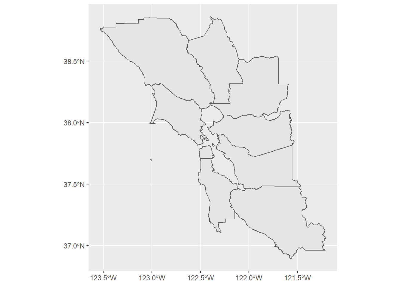

Next, I’ll demonstrate places() which is also from tigris and loads in what we generally would consider to be “cities”. Again, you are only able to load in a full set of cities in a state at a time. This time, let’s use spatial join techniques to filter to just the cities in the Bay Area.

ca_cities <- places("CA", cb = T, progress_bar = FALSE)

We’ve used brackets before to subset dataframes by rows and columns. A neat trick with sf objects is to use brackets to filter one collection of geometries to only those objects that intersect with geometries from another sf object, as shown below:

bay_cities <- ca_cities[bay_counties, ]

mapview(bay_counties, alpha.regions = 0) + mapview(bay_cities)

You should understand this to be a specialized use of brackets; otherwise, brackets are about subsetting by rows and columns. This is simple and quick, but the only problem is that this intersection approach will also retain cities that are just barely touching the boundary of a county but for all intents and purposes should NOT be considered within the counties. The simple solution to this is often to join based on the centroids of the cities. The following pipeline has multiple seemingly serpentine steps but achieves that effect:

bay_cities_within <-
  ca_cities %>% 
  st_centroid() %>% 
  .[bay_counties, ] %>% 
  st_drop_geometry() %>% 
  left_join(ca_cities %>% select(GEOID)) %>% 
  st_as_sf()

mapview(bay_counties, fill = "white", alpha.regions = 0) + mapview(bay_cities_within, label = "NAME")

Notes:

• .[bay_counties, ] is effectively the same as the previous chunk, but in a pipeline, if it’s never obvious how you are asking the pipeline to “receive” the object being passed along, you can use a . as a stand-in (this would also be the case if a function in the pipeline shouldn’t receive the object as its first argument, in which case you put a . wherever you intend it to be received).
• left_join() is one of another set of standard dplyr methods well-explained here. Here, since we want to get the original polygon geometries back which we lost in the pipeline, we left_join() the object in the pipeline to what we started with, ca_cities (with a select() appended, more on that soon), which will add back the original geometry field, but the “leftiness” of the left_join() means that we will only keep the rows that match the pipeline object (which should just be cities in the Bay Area).
• The select() appended to ca_cities removes lots of redundant fields that will become unnecessary duplicates in the result of the left_join() (they also mess things up by renaming the duplicate fields something.x and something.y). With a join, you just need one matching field name, which in this case is self-evidently GEOID. However, note that if you select() on an sf object, it will by default still always hold onto the geometry field, so in this case the object we’re supplying to left_join() has two fields, GEOID and geometry. Only st_drop_geometry() directly removes the geometry field from an sf object.

Here is a shorter way that achieve the same effect, but using some more convoluted filtering methods that may be harder to follow, but I encourage you to try to reverse engineer what’s happening here:

bay_cities_within <-
  ca_cities[which(ca_cities$GEOID %in% st_centroid(ca_cities)[bay_counties, ]$GEOID), ]

If you follow the logic here, this could be a rare case where you choose the non-pipe approach over the pipeline approach, but the two approaches are close enough in time to type. Two mapview outputs were provided above. The following more-stylized leaflet map shows, in green, the bay_cities_within results, and in red, the results from bay_cities that weren’t members of bay_cities_within (note the ! in the filter used like “not”):

leaflet() %>% 
  addTiles() %>% 
  addPolygons(
    data = bay_counties,
    fill = F,
    weight = 2,
    label = ~NAME
  ) %>%
  addPolygons(
    data = bay_cities %>% 
      filter(!GEOID %in% bay_cities_within$GEOID),
    color = "red",
    label = ~NAME
  ) %>% 
  addPolygons(
    data = bay_cities_within,
    color = "green",
    label = ~NAME
  )

Our centroid approach removed some cities clearly outside of the border of the Bay Area counties, like Davis. Note that ~ refers to a field from the dataframe that’s in the pipeline of the leaflet operations.

Our last example in this section will be census block groups (CBGs), which are the most granular geography for Census ACS data. Again, you can pull either official tigris geometries, or use MTC’s clipped geometries. For block_groups() in tigris, you can get CBGs from a set of counties as follows:

bay_cbgs <- block_groups("CA", bay_county_names[1:9], cb = T, progress_bar = F)

I’ll also use this as an opportunity to demonstrate a more generalizable looping technique, map_dfr(), part of the purrr package in tidyverse that is faster than for loops but requires a specific structure. Using this format, map_dfr() takes what’s in the pipe as similar to what you put inside of a for(), what’s between the curly brackets gets looped through the candidates, and the result automatically gets binded together into a dataframe:

bay_cbgs <- 
  bay_county_names %>% 
  map_dfr(function(county) {
    block_groups("CA", county, cb = T, progress_bar = F)
  })

You’d use a technique like this if block_groups() did not let you provide the list of County names directly as an argument.

By the way, instead of using tigris for counties, cities, and CBGs, you could use clipped geometries from the Metropolitan Transportation Commission’s Open Data site (MTC, along with the Association of Bay Area Governments ABAG, are the Bay Area’s regional planning entities, commonly now referred to as Bay Area Metro). Similar to our experience with the CDC 500 Cities dataset, these open data platforms tend to have easy URLs for loading into R. For geometries, generally you should be looking for Shapefiles (an ArcGIS format) or GeoJSONs. The easiest solution is to use st_read() on either type, as shown below (using the URL found under APIs):

bay_cbgs_clip <- st_read("https://opendata.arcgis.com/datasets/037fc1597b5a4c6994b89c46a8fb4f06_0.geojson")

ggplot(bay_cbgs_clip)+geom_sf()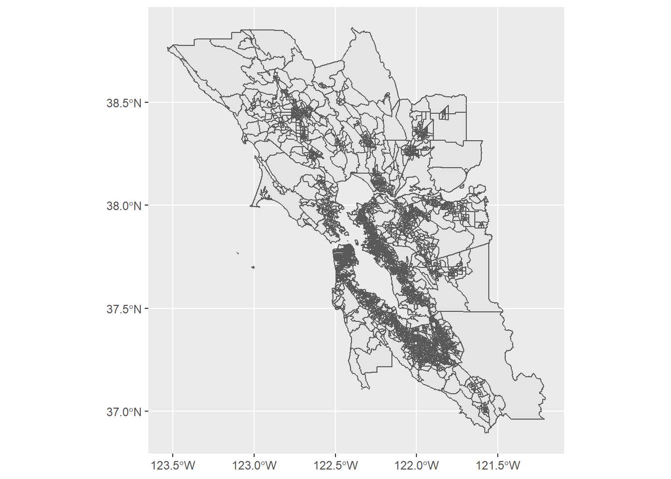

st_read() will automatically convert Shapefiles or GeoJSONs to sf objects, and st_write() allows you to export a sf object as a variety of formats.

The MTC geometries have better shoreline boundaries, but otherwise the tigris options are pretty satisfactory.

We’ll conclude this chapter by mapping the data we’ve read from the CDC and PG&E in Chapter 1 (refer back to code there if you need to read in the relevant datasets again). The PG&E data is provided at the ZIP code level; ZIP codes don’t have official polygon boundaries because they’re ultimately based on collections of point addresses, but the Census Bureau has ZIP code tabulation areas (ZCTAs) that approximate ZIP code boundaries using Census blocks. tigris lets you load ZCTAs for the U.S.

usa_zips <- 
  zctas(cb = T, progress_bar = F)

bay_zips <-
  usa_zips %>% 
  st_centroid() %>% 
  .[bay_counties, ] %>% 
  st_drop_geometry() %>% 
  left_join(usa_zips %>% select(GEOID10)) %>% 
  st_as_sf()

pge_20_res_elec <-
  pge_20_elec %>% 
  filter(CUSTOMERCLASS == "Elec- Residential") %>% 
  mutate(
    ZIPCODE = ZIPCODE %>% as.character()
  ) %>% 
  group_by(ZIPCODE) %>% 
  summarize(
    TOTALKWH = sum(TOTALKWH, na.rm = T)
  ) %>% 
  right_join(
    bay_zips %>% select(GEOID10),
    by = c("ZIPCODE" = "GEOID10")
  ) %>% 
  st_as_sf() %>% 
  st_transform(4326)

Notes:

• I use mutate() to convert ZIPCODE from a double type field to a character type field, since GEOID10 in the other dataframe is a character type field. You can check types using class(pge_20_elec$ZIPCODE). Similar to matching coordinate systems, it doesn’t really matter which option you match to, but for these types of IDs I’d recommend character just in case you ever have leading 0’s that need to be preserved.
• Here, I do a right_join() instead of a left_join(). The joining aspect is the same; the only difference is whether you are retaining the “left side” (e.g. what you have in the pipeline) or the “right side” (e.g. what you are bringing in) of the join. You can think of this as a matter of how many rows the left object has, and how many rows the right object has; the result will have the same number of rows as one of these two objects. In this case, the object in the pipeline has as many ZIP codes as there are in the whole PG&E territory, while bay_zips has just the ZIP codes in the Bay Area. If you do a left_join() here, you’ll still have a dataframe with the energy data, but you would not have gotten a “join” of geometry for any ZIP codes other than the ones in the Bay Area, so the non-Bay ZIP code rows will have “empty geometries” under the geometry field. This actually can still be used for the following mapping step; the non-Bay ZIP data simply won’t be mapped because they won’t have any geometries. But since all you conceptually want is the Bay ZIP code rows to remain, right_join() will conveniently do that for you. There are other kinds of joins as well, which you can learn about when, in the future, you encounter a situation where you conceptually want a different kind of join result.
• In the right_join(), just as you can do in a left_join(), I provide a more complicated argument by = c("ZIPCODE" = "GEOID10") to clarify which fields to join by, since they have different field names. You could adjust these field names in advance, but sometimes it’s easier to just do it in the join step, like this.

Here’s a map of the result, with many more features added to the leaflet map:

res_pal <- colorNumeric(
  palette = "Blues",
  domain = 
    pge_20_res_elec$TOTALKWH
)

leaflet() %>% 
  addTiles() %>% 
  addPolygons(
    data = pge_20_res_elec,
    fillColor = ~res_pal(TOTALKWH),
    color = "white",
    opacity = 0.5,
    fillOpacity = 0.5,
    weight = 1,
    label = ~paste0(
      round(TOTALKWH), 
      " kWh total in ",
      ZIPCODE
    ),
    highlightOptions = highlightOptions(
      weight = 2,
      opacity = 1
    )
  ) %>% 
  addLegend(
    data = pge_20_res_elec,
    pal = res_pal,
    values = ~TOTALKWH,
    title = "Total Residential<br>kWh, 2020"
  )

Notes:

• res_pal is a color palette manually optimized for the range of values in TOTALKWH, using techniques explained here.
• You’re encouraged to play with all the arguments in addPolygons() to understand all the various visual options available.

And here’s the same workflow for the CDC data, specifically mapping the census tract version of “Physical health not good for 14+ days among adults aged 18+ years”, using census tracts from tigris which are a bit bigger than census block groups:

ca_tracts <- tracts("CA", cb = T, progress_bar = F)

bay_phys_health_18 <-
  health_ca %>% 
  filter(
    Measure == "Physical health not good for >=14 days among adults aged >=18 years",
    Year == 2018
  ) %>% 
  left_join(
    ca_tracts %>% select(GEOID),
    by = c("LocationName" = "GEOID")
  ) %>% 
  st_as_sf() %>% 
  st_centroid() %>% 
  .[bay_counties, ] %>% 
  st_drop_geometry() %>% 
  left_join(
    ca_tracts %>% select(GEOID),
    by = c("LocationName" = "GEOID")
  ) %>% 
  st_as_sf()

health_pal <- colorNumeric(
  palette = "Purples",
  domain = 
    bay_phys_health_18$Data_Value
)

leaflet() %>% 
  addTiles() %>% 
  addPolygons(
    data = bay_phys_health_18,
    fillColor = ~health_pal(Data_Value),
    color = "white",
    opacity = 0.5,
    fillOpacity = 0.75,
    weight = 1,
    label = ~paste0(
      round(Data_Value), 
      "% in ",
      LocationName
    ),
    highlightOptions = highlightOptions(
      weight = 2,
      opacity = 1
    )
  ) %>% 
  addLegend(
    data = bay_phys_health_18,
    pal = health_pal,
    values = ~Data_Value,
    title = "Physical health<br>not good for 14+ days<br>among adults aged<br>18+ years, 2018"
  )